Easy Electrical

Featured

LSB Image Steganography Software

Introduction.

In general, Steganography is a process of hiding confidential information in some another form. Then it can be stored in any form.

Simplest example of that can be an envelop. Before sending any confidential files to someone, we envelop those file so others cannot view it.

In this project we’ll store information in the form of BMP (Bit Map) image which is highly uncompressed image. We will take MSB from our message and store it into LSB of Image.

An image consists of multiple pixel. One pixel is of 3 bytes those 3 bytes are nothing but BGR (Blue Green Red) values. So therefore B is of width 1byte, G is of width 1byte and R is of width 1byte.

Why LSB Image Steganography and not MSB?

Hiding data means, it should not be accessible to anyone. Only whoever is authorized he should only be able to access it. Also unauthorized person should not be able to detect that any message (confidential information) is hidden in image.

So, if we change MSB of a byte it will have huge impact on BGR values.

Eg:

If we take a unsigned character variable, it has 8 bits.

Let us asume it has value 128 (ie 1000 0000 in binary). Now here if we modify LSB bit by setting it to 1 its value of that variable will change to 129 (ie 1000 0001) and if we clear (set MSB to 0) MSB value will change from 129 to 1 (0000 0001).

So from this we can observe if we modify the MSB bit there will be huge noticeable change in color of new image and previous image. Whereas on other hand if we change only LSB bits there is no noticeable change in color of image.

Basically, our objective is to encode the text message in image without changing the actual image.

Project Zip

So here I have used C++ with Qt framework to create this project. I’m providing a setup file which you can install and use.

Note: This software will work only on windows.

It is optimised for 1080p resolution.

Download Zip file from here:

https://drive.google.com/file/d/1wUj54lDrwRuYJ2ZRKAwVT0vvNPA1-T4L/view?usp=drive_link

Steps to install:

Extract Zip file and click installer: if you get following message click run anyway.

2. Following window will pop up just click next:

3. Shortcut on desktop will be created double click it:

4. Do following Steps shown in image:

5. Do following Steps shown in image:

6. Do following Steps shown in image:

7. Do following Steps shown in image:

8. Do following Steps shown in image:

9. Do following Steps shown in image:

Click Start encoding to encode message.

10. Do following Steps shown in image:

11. Do following Steps shown in image:

12. Do following Steps shown in image:

13. Do following Steps shown in image:

Featured

Sampling of Continuous Time Signal in MATLAB

The process of converting CT (continuous time) signal to discrete time signal is known as sampling. Sampling is very much necessary for digital systems because a computer cannot understand continuous time signals and sampling is the first step to convert any signal to its digital form.

Simplest form of sampling:-

Above figure shows the simplest process of obtaining samples through a high speed electronic switch. At the input side of switch a CT signal is applies and at the out put we obtain the sampled (discrete time) version of the signal applied at the input.

This is obtained by closing and opening the electronic switch at very high frequency known as sampling frequency.

Sampling frequency is the frequency at which switch is closed and opened is known as sampling frequency.

According to nyquist theorem the sampling frequency should be at least 2 times of fundamental frequency of the signal to be sampled.

Fs=2*Fm

where,

Fs= Sampling Frequency.

Fm= Fundamental frequency.

Sampling With Impulse Signal:-

Above shown is the impulse signal for discrete time.

If we create an impulse train from – infinite to + infinite and multiply the same to a CT signal then also we can convert a signal from CT to DT signal.

Figure below shows impulse train:-

Figure below shows Sampling with impulse train:-

In the figure above x(t) is input CT signal and p(t) is impulse train both of this signals are applied to multiplying box output xs(t)= x(t)*p(t).

The formula for impulse train is:-

By the property of impulse

δ(t−t0)∗x(t)=x(t0)∗δ(t)

Therefore for impulse train:

The code for the same is given below:-

close all;
clc;
clear all;

% Sampaling Frequency and defining time axes
fs=1000;
t=-1:1/fs:1-(1/fs);
f=1;

%General Variables
w=2*pi*f;
a=0;

% Impulse Signal
d=@(t) t==0;

% Sinc Function as CT Signal
syn=@(t) sinc(2*pi*f*t);
figure
plot(t,syn(t));



fss=100;         %Sampling Freq (Number of Impulse that are desired in Impulse train)

T=1/fss; % Sampling Interval

%Creation of Impulse Train
for i=-1:T:1 % for Impulse Train
a=a+d(t-i);
end
%Plotting Impulse Train
figure;
plot(t,a);
title('impulse Train')

%Sampling of a signal with Impulse Train
a=a.*syn(t); % Multiplication of Impulse train with Sinc function

%Plotting of Sampled Signal
figure;
plot(t,a);
title('Impulse Train Multiplied with Sinc');

Below shown is figure of Sinc function:-

Sinc= Sin(wt)/wt;

Below shown is the figure of impulse train:-

Figure shown below is sampled sinc signal:-

Here our x(t) is sinc function

Featured

Creating Signals in MATLAB

Signals are the physical quantity that varies with time. Some standard signals are very important to know behaviour of the system those signals are:

Unit Impulse.
Unit Step.
Ramp.
Sinusoidal.
Sinc.
Signum.

In this blog we are going to create above mentioned signals creating anonymous function of each of them. These signals are also helpful for control system.

For more detail about anonymous function visit: https://www.mathworks.com/help/matlab/matlab_prog/anonymous-functions.html

Here we are creating time axis from -1 to 1 with the step size equal to 1/(sampling frequency). Higher is the sampling frequency better is the signal (but don’t keep sampling frequency too higher because large number of samples requires large amount of processing power so it might take long time to process results) according to nyquist theorem.

Here we are plotting continuous time signal using plot() function. But in case Discrete time plot is needed one can use stem() function instead of plot() in the code. Also here I have used subplot so that all signals are visible on single sheet. One can also plot each function individually using “figure” and “plot();”.

close all;
clc;
clear all;

% Sampling Frequency and defining time axes
fs=1000;
t=-1:1/fs:1-(1/fs);
f=1;

% General Variables
w=2*pi*f;



% Functions
d=@(t) t==0;              %Impulse.
u=@(t) t>=0;              %Unit step.
x=@(t) u(t+0.5)-u(t-0.5); %Rect using unit step.
sn=@(t) sin(2*pi*f*t);    %SineWave.
cs=@(t) cos(2*pi*f*t);    %CosineWave.
tn=@(t) tan(2*pi*f*t);    %TanWave.
rt=@(t) t;                %ramp.
syn=@(t) sinc(2*pi*f*t);  %Sinc.
sng=@(t) 2*u(t)-1;        %Signum.

%ploting
r=3; %subplot rows
c=4; %subplot column

subplot(r,c,1)
plot(t,u(t));
title('unit step');

subplot(r,c,2)
plot(t,sn(t));
title('sine');

subplot(r,c,3)
plot(t,cs(t));
title('cosine');

subplot(r,c,4)
plot(t,tn(t));
title('tan');

subplot(r,c,5)
plot(t,rt(t));
title('ramp');

subplot(r,c,6)
plot(t,syn(t));
title('sinc');

subplot(r,c,7)
plot(t,d(t));
title('impulse');

subplot(r,c,8)
plot(t,sng(t));
title('signum');

subplot(r,c,[10,11])
plot(t,x(t));
title('rect using unit step');

The output of the code after execution is shown in the figure below:-

Featured

AC Current Measurement using Arduino Uno

In this project, we are using current transformer as current sensor. Current Transformer is a device/machine which converts high current from primary to low current at secondary winding which can be easily in proportion to transformation ratio.

Current transformer has two windings primary and secondary, generally primary winding has single turn and secondary has large number of turns.

Transformation ratio = Ipri/Isec=Nsec/Npri

Ipri = primary current

Isec = secondary current

Npri = primary Turns

Nsec = secondary Turns

Current transformer used in this project is ZMPT103C which has turns ratio of 1:1000 that means one turn on primary and 1000 turns on secondary. ZMPT103C is capable to measure current up to 10A (on primary) which produce 10mA on secondary.

The mains wire either phase or neutral needs to be passed through the hole of above ZMCT103C. This mains wire acts as primary of CT. The leads brought out are from secondary of CT.

Caution : Never pass current through primary of CT when secondary is open circuited.

Always keep burden resistance connected across secondary of CT.

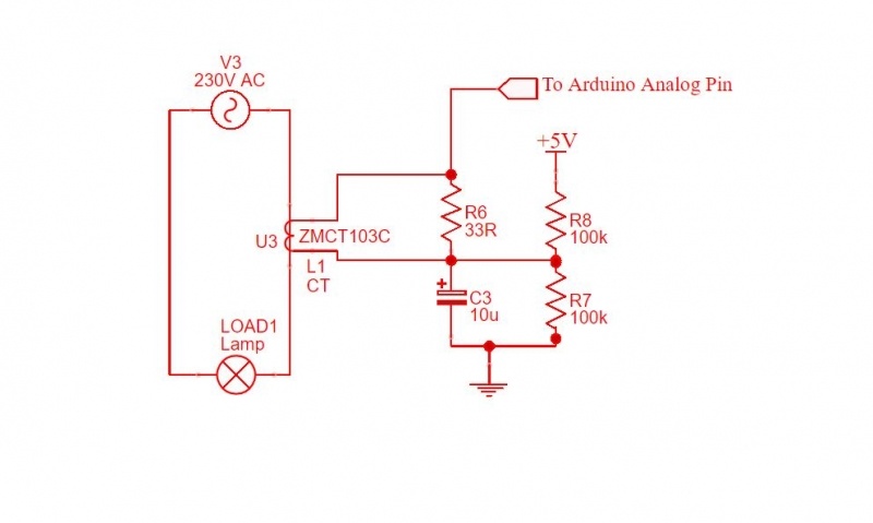
Here we use burden resistance of 33ohm.

Connect CT as shown in below figure.

ZMCT103C Micro Current Transformer | 5A / 5m | Arduino Code

In above figure R6 is used as burden resistance R8 and R7 is used as potential divider. The voltage across burden resistor is AC but microcontroller can recognize DC only so as to shift the AC voltage above ground level we connect one of terminal of CT in between R8 and R7, where as other terminal of CT goes to analog pin A1 of Arduino Uno (or ATMEGA328P). C3 is smoothing capacitor.

Now, whenever 5Amp of current flows from primary 5mA flows from secondary (calculated using transformation ratio). This secondary current produces voltage drop of V_burden =5mA*33ohm. (ohms law V=I*R)

Therefore, we get V_burden =165mV this voltage (AC) +2.5V(DC from potential divider) is fed to analog pin A1 of Arduino therefore voltage received by analog pin when 5 Amp current flows is 2.665V.

To make calculation easy we include emon library in our Arduino code. To install emon library in code you need to install it first to install, open the Library Manager in the Arduino IDE and install it from there. (Make sure your computer is connected to internet while installing.)

Arduino code for measuring current up to 10 amp current 50Hz is:


#include "EmonLib.h"                   // Include Emon Library
EnergyMonitor emon1;                   // Create an instance

void setup()
{  
  Serial.begin(9600);
  
  emon1.current(1, 27.59);             // Current: input pin, calibration.
}

void loop()
{
  double Irms = emon1.calcIrms(1480);  // Calculate Irms only
  

  Serial.println(Irms);          // Irms
}

Relay interfacing with Arduino

In this project we will interface relay to Arduino board. The relay is very useful element when it comes to operate switching A.C.(alternating current) or high power DC devices with micro controller. Relay are of many types and are available in wide range of actuating voltage i.e. 5V, 9V, 12V and so on.

Though arduino is capable to give 5V at its pins but ability to supply current is upto 40-50mA only and most of relay coil require current from 70-100mA. So if we directly connect relay to Arduino then micro controller may get damaged permanently. So to avoid harmful operation we connect a transistor (acting as switch) mostly NPN in common emitter configuration.

The circuit schematics are as bellow:-

Relay interfacing with push button control.

In above shown circuit we have used 5 volt relay which has resistance of 70 ohm. Therefore current drawn by relay can be given by ohms law as:-

I=5v/70ohm =71.42mA of current will be drawn by relay. Therefore we use BC547 NPN transistor which has ability to handle about of 100mA of collector current (obtained from datasheet).

Now because there is inductive coil in relay it has ability to store energy. So as to freewheel this energy freewheeling diode[F.D.] is used.

The LED is connected for observing operation of relay. LED is connected between common and NO(Normally Open) contact of relay supplied by 12V. Current limiting resistor (of atleast 1K) must be connected in series with LED to avoid harmful operation.

Relay coil is connected in collector terminal of transistor. The emitter terminal is connected to ground of Arduino and base terminal of transistor is connected to pin 13 of Arduino board through an 1K current limiting resistor.

At pin 7 push button with pull down resistor is connected. Other terminal of push button is connected to 5V of Arduino.

Arduino Code:-

const int basepin=13;
//constant variable for transistor base pin
const int buttonpin=7;
//constant variable for button pin
int relaystate;
//relay state either on or off.
void setup() {
pinMode(basepin,OUTPUT); 
//we need output from basepin so configured output.
pinMode(buttonpin,INPUT);
//we need input from button so configured input.
}
void loop() {
digitalWrite(basepin,pushbutton());//write high or low depending on press of pushbutton.   
delay(125);
//delay of 125 ms
}
//function created for push button operation.
int pushbutton(){
int buttonstate=digitalRead(buttonpin);  
if(buttonstate==HIGH){
if(relaystate==LOW){
  relaystate=HIGH; 
}
else{relaystate=LOW;}
}
return relaystate;
  
}

Working of circuit:-

When the push button is pressed for first time micro controller registers the press and relay is turned on and 12 volt appears across series combination of 1K resistor and LED. When same button is pressed second time the relay would turn off and LED will also gets turned off.